W1: Practical exercise 1

library(StatInsQuestions)

Verify through simulation the variance of the approximations of Theorems 1.11 and 1.12

a)

Let $Z_n$ be a sequence of iid r.v. where $Z_n \sim \mathcal{N}(0,1) \, \forall n$. Verify the asymptotic distribution $\sqrt{n}(\bar{\sigma}^2_n - \mu^{(2)})$, where $\mu^{(2)} = E((Z_1 - E(Z_1))^2)$

First we aim to create the various empiric elements:

data <- rnorm(
  n = 1000000, 
  mean = 0, 
  sd = 1
)

mu_2 <- 1
mu_4 <- 3

n <- length(data)
i <- seq_len(n)

cum1 <- cumsum(data)
cum2 <- cumsum(data^2)

m1 <- cum1 / i 
m2 <- cum2 / i 

sigma2_hat_1n <- function(x) 
{
 r <-  mean(x^2) - mean(x)^2
 return(r)
}

simulate_Tn <- function(
    n,
    B = 200
) {
  Z <- matrix(rnorm(n * B), nrow = n, ncol = B)
  m1 <- colMeans(Z)
  m2 <- colMeans(Z^2)
  hatvar <- m2 - m1^2
  sqrt(n) * (hatvar - 1)
}


n <- 10000
B <- 20000
Tn <- simulate_Tn(n , B)

df <- tibble::tibble(Tn = Tn)

And we plot the simulations and compare them with the expected distribution $\mathcal{N}(0,2)$

ggplot2::ggplot(df, ggplot2::aes(Tn)) + 
  ggplot2::geom_density( linewidth = 1) + 
  ggplot2::stat_function(fun = dnorm, args = list(mean = 0, sd = sqrt(2)),
                linewidth = 1, color = "red")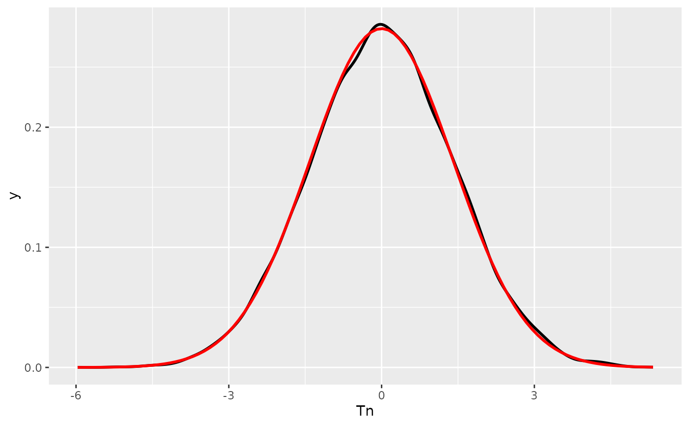 

Which we see aligns nicely.

b)

Let $Z_n$ be a sequence of iid r.v. where $Z_n$ is pareto with shape $\alpha = 3$ and scale $\kappa = 100$ for alle n.  Verify the asymptotic distribution for $u = 200$ of $\sqrt{n}(\mathbb{e_n(u) - e_F(u)})$